Comparing DataFrames
What is data-diff ?
DataFrame (or table) comparison is the most important feature that any SQL-based OLAP engine
should have. I personally use it all the time whenever I work on a data pipeline, and
I think it is so useful and powerful that it should be a built-in feature of any
data pipeline development tool, just like git diff is the most important feature when
you use git.
What does it do ?
Simple: it compares two SQL tables (or DataFrames), and gives you a detailed summary of what changed between the two, letting you perform in-depth analysis when required.
Why is it useful ?
During the past few decades, code diff, alongside automated testing, has become the cornerstone tool used for implementing coding best-practices, like versioning and code reviews. No sane developer would ever consider using versioning and code reviews if code-diff wasn't possible.
When manipulating complex data pipelines, in particular with code written in SQL or DataFrames, it quickly becomes extremely challenging to anticipate and make sure that a change made to the code will not have any unforeseen side effects.
How to get started ?
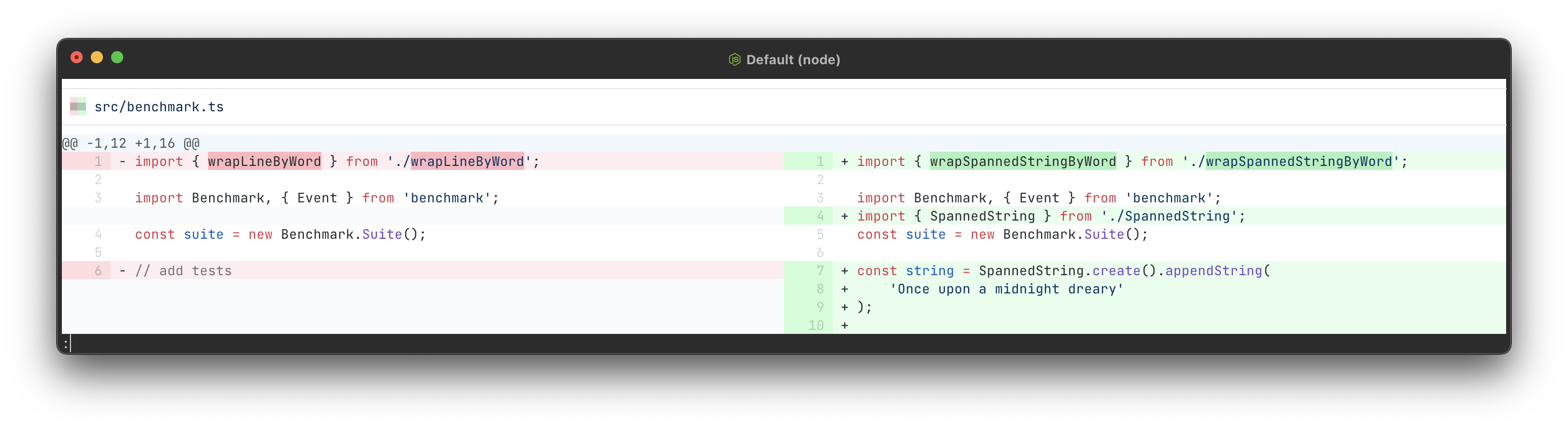
Here is a minimal example of how you can use it :
First, create a PySpark job with spark-frame and data-diff-viewer as dependencies (check this project's README.md to know which versions of data-diff-viewer are compatible with spark-frame)
Then run a PySpark job like this one:
And that's it! After the job has run, you should get an HTML report at the location specified with output_file_path.
The only parameter to be wary of are:
join_cols
join_cols indicates the list of column names that will be used to join the two DataFrame together for the
comparison. This set of columns should follow an unicity constraint in both DataFrames to prevent a
combinatorial explosion.
Features
- If
join_colsis not set, the algorithm will try to infer one column automatically, but it can only detect single columns, if the DataFrames require multiple columns to be joined together, the automatic detection will not work. - The algorithm comes with a safety mechanism to avoid performing joins that would lead to a combinatorial explosion when the join_cols are incorrectly chosen.
output_file_path
The path where the HTML report should be written.
Features
This method uses Spark's FileSystem API to write the report.
This means that output_file_path behaves the same way as the path argument in df.write.save(path):
- It can be a fully qualified URI pointing to a location on a remote filesystem (e.g. "hdfs://...", "s3://...", etc.), provided that Spark is configured to access it
- If a relative path with no scheme is specified (e.g.
output_file_path="diff_report.html"), it will write on Spark's default's output location. For example:- when running locally, it will be the process current working directory.
- when running on Hadoop, it will be the user's home directory on HDFS.
- when running on the cloud (EMR, Dataproc, Azure Synapse, Databricks), it should write on the default remote storage linked to the cluster.
Methods used in this example
spark_frame.data_diff.compare_dataframes
Compares two DataFrames and return a DiffResult object.
We first compare the DataFrame schemas. If the schemas are different, we adapt the DataFrames to make them as much comparable as possible: - If the order of the columns changed, we re-order them automatically to perform the diff - If the order of the fields inside a struct changed, we re-order them automatically to perform the diff - If a column type changed, we cast the column to the smallest common type - We don't recognize when a column is renamed, we treat it as if the old column was removed and the new column added
If join_cols is specified, we will use the specified columns to perform the comparison join between the
two DataFrames. Ideally, the join_cols should respect an unicity constraint.
If they contain duplicates, a safety check is performed to prevent a potential combinatorial explosion:
if the number of rows in the joined DataFrame would be more than twice the size of the original DataFrames,
then an Exception is raised and the user will be asked to provide another set of join_cols.
If no join_cols is specified, the algorithm will try to automatically find a single column suitable for
the join. However, the automatic inference can only find join keys based on a single column.
If the DataFrame's unique keys are composite (multiple columns) they must be given explicitly via join_cols
to perform the diff analysis.
Tips
- If you want to test a column renaming, you can temporarily add renaming steps to the DataFrame you want to test.
- If you want to exclude columns from the diff, you can simply drop them from the DataFrames you want to compare.
- When comparing arrays, this algorithm ignores their ordering (e.g.
[1, 2, 3] == [3, 2, 1]). - When dealing with a nested structure, if the struct contains a unique identifier, it can be specified
in the join_cols and the structure will be automatically unnested in the diff results.
For instance, if we have a structure
my_array: ARRAY<STRUCT<a, b, ...>>and ifais a unique identifier, then you can add"my_array!.a"in the join_cols argument. (cf. Example 2)
Parameters:
| Name | Type | Description | Default |
|---|---|---|---|
left_df |
DataFrame
|
A Spark DataFrame |
required |
right_df |
DataFrame
|
Another DataFrame |
required |
join_cols |
Optional[List[str]]
|
Specifies the columns on which the two DataFrames should be joined to compare them |
None
|
Returns:
| Type | Description |
|---|---|
DiffResult
|
A DiffResult object |
Example 1: simple diff
>>> from spark_frame.data_diff.compare_dataframes_impl import __get_test_dfs
>>> from spark_frame.data_diff import compare_dataframes
>>> df1, df2 = __get_test_dfs()
>>> df1.show()
+---+-----------+
| id|   my_array|
+---+-----------+
|  1|[{1, 2, 3}]|
|  2|[{1, 2, 3}]|
|  3|[{1, 2, 3}]|
+---+-----------+
>>> df2.show()
+---+--------------+
| id|      my_array|
+---+--------------+
|  1|[{1, 2, 3, 4}]|
|  2|[{2, 2, 3, 4}]|
|  4|[{1, 2, 3, 4}]|
+---+--------------+
>>> diff_result = compare_dataframes(df1, df2)

Analyzing differences...
No join_cols provided: trying to automatically infer a column that can be used for joining the two DataFrames
Found the following column: id
Generating the diff by joining the DataFrames together using the inferred column: id
>>> diff_result.display()
Schema has changed:
@@ -1,2 +1,2 @@

 id INT
-my_array ARRAY<STRUCT<a:INT,b:INT,c:INT>>
+my_array ARRAY<STRUCT<a:INT,b:INT,c:INT,d:INT>>
WARNING: columns that do not match both sides will be ignored

diff NOT ok

Row count ok: 3 rows

0 (0.0%) rows are identical
2 (50.0%) rows have changed
1 (25.0%) rows are only in 'left'
1 (25.0%) rows are only in 'right

Found the following changes:
+-----------+-------------+---------------------+---------------------------+--------------+
|column_name|total_nb_diff|left_value           |right_value                |nb_differences|
+-----------+-------------+---------------------+---------------------------+--------------+
|my_array   |2            |[{"a":1,"b":2,"c":3}]|[{"a":1,"b":2,"c":3,"d":4}]|1             |
|my_array   |2            |[{"a":1,"b":2,"c":3}]|[{"a":2,"b":2,"c":3,"d":4}]|1             |
+-----------+-------------+---------------------+---------------------------+--------------+

1 rows were only found in 'left' :
Most frequent values in 'left' for each column :
+-----------+---------------------+---+
|column_name|value                |nb |
+-----------+---------------------+---+
|id         |3                    |1  |
|my_array   |[{"a":1,"b":2,"c":3}]|1  |
+-----------+---------------------+---+

1 rows were only found in 'right' :
Most frequent values in 'right' for each column :
+-----------+---------------------------+---+
|column_name|value                      |nb |
+-----------+---------------------------+---+
|id         |4                          |1  |
|my_array   |[{"a":1,"b":2,"c":3,"d":4}]|1  |
+-----------+---------------------------+---+
>>> diff_result.export_to_html(output_file_path="test_working_dir/compare_dataframes_example_1.html")
Report exported as test_working_dir/compare_dataframes_example_1.html
Check out the exported report here
Example 2: diff on complex structures
By adding "my_array!.a" to the join_cols argument, the array gets unnested for the diff
>>> diff_result_unnested = compare_dataframes(df1, df2, join_cols=["id", "my_array!.a"])

Analyzing differences...
Generating the diff by joining the DataFrames together using the provided column: id
Generating the diff by joining the DataFrames together using the provided columns: ['id', 'my_array!.a']
>>> diff_result_unnested.display()
Schema has changed:
@@ -1,4 +1,5 @@

 id INT
 my_array!.a INT
 my_array!.b INT
 my_array!.c INT
+my_array!.d INT
WARNING: columns that do not match both sides will be ignored

diff NOT ok

WARNING: This diff has multiple granularity levels, we will print the results for each granularity level,
         but we recommend to export the results to html for a much more digest result.

##############################################################
Granularity : root (4 rows)

Row count ok: 3 rows

2 (50.0%) rows are identical
0 (0.0%) rows have changed
1 (25.0%) rows are only in 'left'
1 (25.0%) rows are only in 'right

1 rows were only found in 'left' :
Most frequent values in 'left' for each column :
+-----------+-----+---+
|column_name|value|nb |
+-----------+-----+---+
|id         |3    |1  |
|my_array!.a|1    |2  |
|my_array!.b|2    |2  |
|my_array!.c|3    |2  |
+-----------+-----+---+

1 rows were only found in 'right' :
Most frequent values in 'right' for each column :
+-----------+-----+---+
|column_name|value|nb |
+-----------+-----+---+
|id         |4    |1  |
|my_array!.a|1    |1  |
|my_array!.a|2    |1  |
|my_array!.b|2    |2  |
|my_array!.c|3    |2  |
|my_array!.d|4    |3  |
+-----------+-----+---+

##############################################################
Granularity : my_array! (5 rows)

Row count ok: 3 rows

1 (20.0%) rows are identical
0 (0.0%) rows have changed
2 (40.0%) rows are only in 'left'
2 (40.0%) rows are only in 'right

2 rows were only found in 'left' :
Most frequent values in 'left' for each column :
+-----------+-----+---+
|column_name|value|nb |
+-----------+-----+---+
|id         |3    |1  |
|my_array!.a|1    |2  |
|my_array!.b|2    |2  |
|my_array!.c|3    |2  |
+-----------+-----+---+

2 rows were only found in 'right' :
Most frequent values in 'right' for each column :
+-----------+-----+---+
|column_name|value|nb |
+-----------+-----+---+
|id         |4    |1  |
|my_array!.a|1    |1  |
|my_array!.a|2    |1  |
|my_array!.b|2    |2  |
|my_array!.c|3    |2  |
|my_array!.d|4    |3  |
+-----------+-----+---+
>>> diff_result_unnested.export_to_html(output_file_path="test_working_dir/compare_dataframes_example_2.html")
Report exported as test_working_dir/compare_dataframes_example_2.html
Check out the exported report here
Source code in spark_frame/data_diff/compare_dataframes_impl.py
715 716 717 718 719 720 721 722 723 724 725 726 727 728 729 730 731 732 733 734 735 736 737 738 739 740 741 742 743 744 745 746 747 748 749 750 751 752 753 754 755 756 757 758 759 760 761 762 763 764 765 766 767 768 769 770 771 772 773 774 775 776 777 778 779 780 781 782 783 784 785 786 787 788 789 790 791 792 793 794 795 796 797 798 799 800 801 802 803 804 805 806 807 808 809 810 811 812 813 814 815 816 817 818 819 820 821 822 823 824 825 826 827 828 829 830 831 832 833 834 835 836 837 838 839 840 841 842 843 844 845 846 847 848 849 850 851 852 853 854 855 856 857 858 859 860 861 862 863 864 865 866 867 868 869 870 871 872 873 874 875 876 877 878 879 880 881 882 883 884 885 886 887 888 889 890 891 892 893 894 895 896 897 898 899 900 901 902 903 904 905 906 907 908 909 910 911 912 913 914 915 916 917 918 919 920 921 922 923 924 925 926 927 928 929 930 931 932 933 934 935 936 937 938 939 940 941 942 943 944 945 946 947 948 949 950 951 952 953 954 955 956 957 958 959 960 961 962 963 964 965 966 967 968 969 970 971 972 973 974 975 976 977 978 979 980 981 | |
spark_frame.data_diff.DiffResult.export_to_html
Generate an HTML report of this diff result.
This generates an HTML report file at the specified output_file_path URI location.
The report file can be opened directly with a web browser, even without any internet connection.
Info
This method uses Spark's FileSystem API to write the report.
This means that output_file_path behaves the same way as the path argument in df.write.save(path):
- It can be a fully qualified URI pointing to a location on a remote filesystem (e.g. "hdfs://...", "s3://...", etc.), provided that Spark is configured to access it
- If a relative path with no scheme is specified (e.g.
output_file_path="diff_report.html"), it will write on Spark's default's output location. For example:- when running locally, it will be the process current working directory.
- when running on Hadoop, it will be the user's home directory on HDFS.
- when running on the cloud (EMR, Dataproc, Azure Synapse, Databricks), it should write on the default remote storage linked to the cluster.
Parameters:
| Name | Type | Description | Default |
|---|---|---|---|
title |
Optional[str]
|
The title of the report |
None
|
encoding |
str
|
Encoding used when writing the html report |
'utf8'
|
output_file_path |
str
|
URI of the file to write to. |
'diff_report.html'
|
diff_format_options |
Optional[DiffFormatOptions]
|
Formatting options |
None
|
Examples:
>>> from spark_frame.data_diff.diff_result import _get_test_diff_result
>>> diff_result = _get_test_diff_result()
>>> diff_result.export_to_html(output_file_path="test_working_dir/diff_result_export_to_html_example.html")
Report exported as test_working_dir/diff_result_export_to_html_example.html
Check out the exported report here
Source code in spark_frame/data_diff/diff_result.py
How to read it ?
Once the report is generated, you can simply open it with any browser and you will see a web page with three sections:
-
A title headline
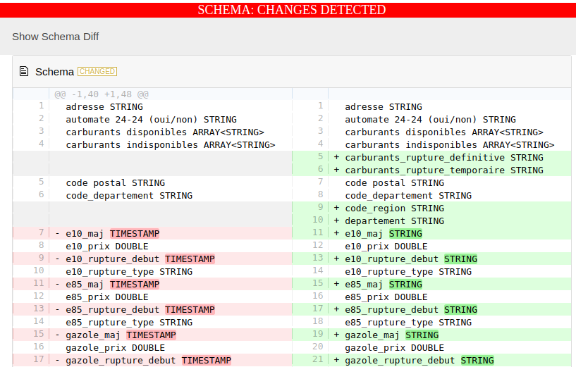
-
A schema diff that should look like this:
- And a data-diff that should look like this:
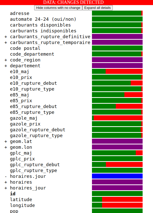
The data diff reads like this:
- There is one line per column in the DataFrame.
- If a column does not exist in the first DataFrame, it will be prefixed with a
+and the bar will be purple. - If a column does not exist in the second DataFrame, it will be prefixed with a
-and the bar will be blue. - Otherwise, the bar chart represent the percentage of rows that are identical (in green) vs. the percentage that differ (in red).
You can interact with the data diff by mousing over and clicking on the bar charts:
-
If you mouse over a bar chart, a detailed percentage and count of each type of value will appear:
-
If you click on a bar chart, a detail of the most frequent changes and non-changes will appear :
-
You can then click on the details to display a full example of row comparison where this change/non-change happens:
-
Clicking on the line that is already selected will make the full example disappear
-
On top of the data diff, there are also two buttons: "Hide columns with no change" and "Expand all details", which are useful when you need to focus on reviewing all the changes in a data-diff:
Examples
Simple examples
Some simple examples are available in the reference of the method spark_frame.data_diff.compare_dataframes.
French gas price
We made a notebook using a real complex use-case using Open Data.
You can open it directly in Google Colab using this link:
![]()
Or if you don't want to use Google Colab, you can open it directly in github.
If you're in a hurry, here are two examples of diffs generated with this notebook:
- Diff obtained in the middle of the cleaning process
- Diff obtained at the end, before analysis of the remaining differences
What are some common use cases ?
From the simplest to the most complex, data-diff is super useful in many cases :
Refactoring a single SQL query
Refactoring a single SQL query is something I do very often when I get my hand on legacy code. I do it quite often in order to :
- Improve the readability of the code.
- Get to know the code better ("why is it done like this and not like that ?").
- Improving the performances.
Usually, the results of the refactoring process will be a new query which is much cleaner, more efficient, but produces exactly the same result.
That's when data-diff becomes extremely handy, as it can make sure the results are 100% identical.
Funny story: more than once, after refactoring a SQL query, I noticed small differences in the results thanks to data-diff.
After further inspection I sometimes realized that my refactoring had introduced a new bug, but other times
I realized that my refactoring actually fixed a bug that was previously existing and went unnoticed until then. 
But of course, what we said also applies to data transformations written with DataFrames, and also to whole pipelines chaining multiple transformations or queries.
Refactoring a whole data pipeline
Refactoring a data pipeline is often one of the most daunting and scary tasks that an Analytics Engineer has to carry. But there are many good reasons to do it, such as:
- To reduce code duplication (when you realise that the exact same CTE appears in 3 or 4 different queries)
- To improve maintainability, readability, stability, documentation, testing: if a query contains 20 CTEs, it's probably a good idea to split it in smaller parts, thus making the intermediary results easier to document, test and inspect.
- For many other cases listed below in dedicated items
Here again, when we do so we want to make sure the results are exactly the same as they were before.
Fixing a bug in a query
Whenever I work on a fix, I use data-diff to make sure that the changes I wrote have the exact effect I was planning to have on the query and nothing more. I also make sure that this change does not impact the tables downstream.
Example
Here is a very simple example of a fix that could go wrong: you notice one of your type has a column country
that contains the following value counts:
| direction | count |
|---|---|
| FRANCE | 124 590 |
| france | 4 129 |
| germany | 209 643 |
| GERMANY | 1 2345 |
Note
As this is a toy example, we won't go far into the details of why such things happened in the first place. Let's imagine you work for a French company that bought a German company, and you are merging the two information systems, and that at some point the prod platform was updated to make sure only UPPERCASE was used. Needless to stress the importance of making sure that your input data is of the highest possible quality using data contracts...
You decide to apply a fix by passing everything to uppercase, adding a nice "SELECT UPPER(direction) as direction"
somewhere in the code, ideally during the cleaning or bronze stage of your data pipeline. (Needless to say, it would
be even better if the golden source for your data were fixed and backfilled, or even better if that inconsistency
never happened in the first place, but that kind of perfect solution requires a strong commitment at every level of your
organisation, and the metrics in your CEO's dashboard needs to be fixed today, not in a few months...)
So you implement that fix, and run data-diff to make sure the results are good. You get something like this:
136935 (39.0%) rows are identical
213772 (61.0%) rows have changed
0 (0.0%) rows are only in 'left'
0 (0.0%) rows are only in 'right

Found the following changes:
+-----------+-------------+---------------------+---------------------------+--------------+
|column_name|total_nb_diff|left_value           |right_value                |nb_differences|
+-----------+-------------+---------------------+---------------------------+--------------+
|direction  |213772       |germany              |GERMANY                    |209643        |
|direction  |213772       |france               |FRANCE                     |4129          |
+-----------+-------------+---------------------+---------------------------+--------------+
With this, you are now 100% sure that the change you wrote did not impact anything else... at least on this table. Let's say that you now recompute this table and use data-diff on the table downstream, and you notice that one of your tables (the one that generates the CEO's dashboard) has the following change:
136935 (39.0%) rows are identical
213772 (61.0%) rows have changed
0 (0.0%) rows are only in 'left'
0 (0.0%) rows are only in 'right

Found the following changes:
+------------+-------------+---------------------+---------------------------+--------------+
|column_name |total_nb_diff|left_value           |right_value                |nb_differences|
+------------+-------------+---------------------+---------------------------+--------------+
|country_code|213772       |DE                   |NULL                       |209643        |
|country_code|213772       |NULL                 |FR                         |4129          |
+------------+-------------+---------------------+---------------------------+--------------+
Now, that change is unexpected. So you go have a look at the SQL query generating this dashboard, and you notice this:
SELECT
    ...
    CASE
        WHEN country = "germany" THEN "DE"
        WHEN country = "FRANCE" THEN "FR
    END as country_code,
    ...
Now it all makes sense! Perhaps the query used to be "correct" at some point in time when "germany" and "FRANCE" were the only possible values in that column, but this is not the case anymore. And by fixing one bug upstream, you had unforeseen impacts on the downstream tables. Thankfully data-diff made it very easy to spot !
Note
Of course, upon reading this, any senior analytics engineer is probably thinking that many things went wrong
in the company to lead to this result. Indeed. Surely, the engineer who wrote that CASE WHEN statement should
have performed some safety data harmonization in the cleaning stage of the pipeline. Surely, the developers of
the data source never should have sent inconsistent data like this. But nevertheless that kind of scenario (and
much worse ones) often happens in real life, especially when you arrive in a young company that
"go fast and break things" and you inherit the legacy of your predecessors.
Implementing a new feature
Sometimes I am tasked with adding a new column, or enriching the content of an existing column. Once again, data-diff makes it very easy to make sure that I added the new column in the right place and that it contains the expected values.
Reviewing other's changes
Code review is one of the most important engineering best practices of this century. I find that some data teams still
don't do it as much as they should, but we are getting there. dbt did a lot for the community to bring engineering
best-practices to the data teams. What makes code reviews even better and easier, is when a data-diff comes with
it. DataDiffResults can be exported as standalone HTML reports, which makes them very easy to share to others,
or to post in the comment of a Merge Request. If your DataOps are good enough, they can even automate the whole
process and make your CI pipeline generate and post the data-diff report automatically for you.
If you prefer premium tech rather than building things yourself, I strongly suggest you have a look at DataFold who provides on-the-shelf CI/CD for data teams, including a nice data-diff feature.
Note
At this point, you are probably wondering why I went all the way to make my own data-diff tool, if I recommend trying another paying tool that already does it on the shelf. Here a few elements of response:
- Spark-frame is 100% free and open-source.
- Datafold does have an open-source data-diff version, but it is much more limited (and does not generate HTML reports). If I ever have the time, I will make a detailed feature comparison of both data-diffs.
- I believe spark-frame's data-diff is more powerful than Datafold's premium data-diff version, because it works well with complex data structures too.
- I hope people will use spark-frame's (and bigquery-frame's) data-diff to build up more nice features to easily have a full data-diff integration in their CI/CD pipelines.
See what changed in your data
When receiving full updates on a particular dataset. Data-diff can be simply used to display the changes that occurred between the old and new version of the data.
This can be useful to troubleshoot issues, or simply to know what changed.
However, this not the primary use-case we had in mind when making data-diff, and some other data-drift monitoring tools might be better suited for this (like displaying the number of rows added per day, etc.).
Even though, advanced users might want to take a look at the
DiffResult.diff_df_shards attribute
that provides access to the whole diff DataFrame, which can be used to retrieve the
exact set of rows that were updated, for instance.
Releasing your data-models to prod like a pro
For me, the Graal  of analytics engineering best practices is to achieve full versioning of your data model.
Just like well-maintained libraries are fully versioned.
of analytics engineering best practices is to achieve full versioning of your data model.
Just like well-maintained libraries are fully versioned.
That would mean that every table you provide to your users has a version number. Whenever you introduce a breaking change in the table's schema or data, you increase the minor version number (and you keep the major version for full pipeline overhauls). You then maintain your pipelines for multiple versions, and leave the time for your users to catch up with the changes before decommissioning the older versions.
Of course, this is quite difficult to achieve in practice because:
- It's complicated to put in place:
- It can be very costly:
- If your data warehouse already costs you an arm, then maintaining two or more versions of it would cost as many more limbs. This is clearly not feasible when you are trying to optimize costs.
One simpler alternative to versioning exists, it is called Blue-Green deployment. It is a concept used in infrastructure deployment but the idea can be adapted to data pipelines. The main advantage is that it limits the number of versions of your data to 2. But it means that you need your users to adapt to the new version quickly before being able to continue pushing new breaking changes.
Whichever strategy you choose, versioning or blue-green, I believe it would be extremely valuable for end users to get release notes whenever a model evolves, and if those notes showed you exactly which table changed and how. Not only for the table's schema but also for the table's data. That would be, for me, the apex of analytics engineering best practices.